Introduction to Recommender Systems

Recommender Systems (RS) are software applications that provide a list of suggestions to users. For instance, YouTube provides a list of recommended videos according to user’s profile history. Or Amazon website recommends some items based on the end user.

Recommendation systems serve two purposes usually:

To promote or stimulate the user to buy/watch something.
To handle the information overload problem by extracting the information that users require. This is related to Information Filtering (IF), Information Retrieval (IR). The goal is to separate useful materials (items) from non-useful ones which are more relevant to content-based filtering (described later).

Recommender Systems have three main types.

Collaborative filtering
Content-based filtering
Knowledge-based

Collaborative Filtering

Basically, collaborative filtering is the most fundamental recommender system type. In this filtering, the process of recommendation is done by analyzing the user-item matrix (vector) to find the users who have similar tastes. Then based on the similar users’ history, the system will predict the rate of items that active user has not rated yet. In the next step, the system will provide two outputs. One is to what extends the user would like or dislike and then top N items would be provided to the active user. The main idea behind this type of filtering is that if the users in the past have some interests in common, it is likely that they do the same taste in the future.

The pure CF approach does not need to have any knowledge regarding the items, just requires user-item matrix. This provides the advantage that in the system information regarding the items doesn’t need to be entered.

Collaborative filtering has a variety of approaches which are discussed in the following.

User-based nearest neighbor recommendations

In this approach, the id of the active user is provided to the system. Then based on that the system would identify similar users (peer users) that have similar preferences.

Afterward, the system would predict (rate), the rating for each item (P) that active user has not rated (seen) yet.

To provide the recommendation to the active user, the system should first predict the rate for the items that user has not seen yet. Then according to the outcome of ratings of the peers, the system would decide to provide a particular item to the active user or not.

According to what mentioned, the process should be done in three steps.

Identify the peers (similar users) to the active user.
Predict the items ratings.
If prediction rate is high add the item in the recommendation list.

The most basic approach to identify similar peer is to apply Pearson’s Correlation Coefficient function. The function can be defined in such a way that it returns a float number between 1 and -1 to indicate similarity between two users (active $[A]$ and random user $[B]$ ).

$Function float = Sim (A, B)$

The value of the function would be between 1 to -1. Which the former denotes to a strong correlation between two users and the latter implies two users do not share anything.

Following is the Pearson Correlation Coefficient equation

$sim(a,b)=\frac{\sum_{p\epsilon P}({r_{a,p}}-\bar{r}_{a})(r_{b,p}-\bar{r}_{b})}{\sqrt{\sum _{p\epsilon P}(r_{a,p}-\bar{r}_{a})^{2}}{\sqrt{\sum _{p\epsilon P}(r_{b,p}-\bar{r}_{b})^{2}}}}$

$R$ rating

$A$ user $A$

$B$ user $B$

$P$ product/item

The next step is to select the nearest neighbors (peers) for the active user and predict the rating products that active user has not rated yet.

Assume the system defines a threshold to select all a user as a peer if and only if the rate of correlation is more than $\geq 0.70$ and system at least can identify two peers, if not the system would decrease the similarity to 0.50. For more information refer to Neighborhood selection.

Based on what mentioned in the above paragraph the system identified two peer users who are User $J$ and User $K$ respectively. Now in order to predict the rate of Item $X$ for the active user, the system needs a predict function which is following equation.

$pred(a,p)=\bar r_{a} + \frac{\sum _ {b\epsilon N} sim(a,b)*(r_sub{b,p}-\bar{r}_{b})}{\sum _{b\epsilon N}sim(a,b)}$

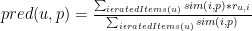
The result of Pred function would be 1 to 5. Recommending an item to a user is usually done by defining a threshold in a flexible manner.

Besides Pearson’s correlation, there are other metrics such as adjusted cosine similarity, Spear’s rank correlation coefficient, or the mean squared difference that can be used to determine the proximity between users. However, empirical analyses show that for user-based recommender systems, the Pearson coefficient outperforms other measures of comparing users. However, for the item-based recommender systems, it has been reported that the cosine similarity measure consistently outperforms the Pearson coefficient.

One the well-known problem of Pearson Correlation is the lack of taking universal items that are liked by everybody. It means the equation does not take into account that some items rating has more value than others [general ones]. One solution to this problem is applying a transformation function to Pearson Correlation which reduces the importance of generally liked items which is called as Inverse user frequency. Or the problem can be settled by Variance weighting factor.

In addition to that Pearson Correlation equation does not take into consideration the number of the items that rated by the users. For instance, active user has rated only 5 items out of $N$ number of items and user $K$ rated 1000 items out of $N$ items but the correlation between these two users would show so strong as the equation only takes the only rating into consideration that active user rated ( this example 5 ratings-only) and dismiss the rest.

Hence, to overcome the mentioned issues, the better weighting approach is called Significance Weighting. In the Significance Weighting, just a threshold is defined for the number of items the user rated, for example, if the less than 50 items are in common the system would be excluded the user. In other words, the active user and user $K$ at least should have 50 items in common which have been rated by both of them. The approach also does not work when the dataset is small and finding $N$ (here 50) number of the co-rated item is difficult.

Finally, another proposal for improving the accuracy of the recommendations by fine-tuning the prediction weights in termed case amplification. Case amplification refers to an adjustment of the weights of the neighbors in a way that values close to +1 and -1 are emphasized by multiplying the original weights by a constant factor $p$ .

Neighborhood selection

There are two approaches to select the neighbors for the active user.

Using threshold, which based on the research it is not effective.
Using K nearest neighbors, which is the better approach. According to the research, the best $K$ number is between 20 to 50 and however, 10 is very few and not good.

Item-based nearest neighbor

When there are millions of items and users in the system, applying user-based CF doesn’t seem logical and it would cause many problems since the data can’t process real-time in large amount. Hence, in order to speed up the processing data section, the data should be pre-processed before which is called offline pre-processing.

The main idea behind item-based nearest neighbor is to identify the similar items and then applying the prediction for the item which user has not rated it yet. To do so, the system identifies the items that received similar ratings, for instance item5 $(1,2,3,4,?)$ is similar with item2 $(5,4,4,3,2)$ and item3 $(4,5,3,5,2)$ . Then in the next step, the system would do the calculation for the unrated item for the active user (in this case item5) based on the history of rating of the active user for the similar items. For example, the active user gave 2 to item5 and item3. Now, if we do the calculation for “?”, the rating would be 2.

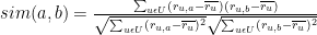
The equation which is used to find similar items is so-called Cosine similarity measure. The equation calculates the similarity between two N-dimensions vector ( $N$ dimensions vector denotes to item-5 and item-3 or item-5 and item-2).

The similarity between two items $a$ and $b$ – viewed as the corresponding rating vectors $\overrightarrow{a}$ and $\overrightarrow{b}$ – is formally defined as follows:

$sim(\overrightarrow{a},\overrightarrow{b})=\frac{\overrightarrow{a}.\overrightarrow{b}}{\left | \overrightarrow{a} \right |*\left | \overrightarrow{b} \right |}$

The $.$ symbol is the dot product of vectors. $\overrightarrow{a}$ is the Euclidian length of the vector, which is defined as the square root of the dot product of the vector with itself.

The cosine similarity of item5 and item1 is therefore calculated as follows:

$sim(I5,I1)=\frac{3*3+5*4+4*3+1*1}{\sqrt{3^{2}+{5^{2}}+{4^{2}}+{1^{2}}}*\sqrt{3^{2}+{4^{2}}+{3^{2}}+{1^{2}}}}=0.99$

The result of Sim function would be between 0 to 1 which 1 indicates to strong similarity and 0 donates to totally different between items.

The possible similarity values are between 0 and 1, where values near to 1 indicate a strong similarity. The basic cosine measure does not take the differences in the average rating behavior of the users into account. This problem is solved by using the adjusted cosine measure, which subtracts the user average from the ratings. The values for the adjusted cosine measure correspondingly range from -1 to +1, as the Pearson measure.

Let $U$ be the set of users that rated both items $a$ and $b$ . The adjusted cosine measure is then calculated as follows:

$sim(a,b)=\frac{\sum _{u\epsilon U}(r_{u,a}-\overline{r_{u}})(r_{u,b}-\overline{r_{u}})}{\sqrt{\sum _{u\epsilon U}(r_{u,a}-\overline{r_{u}})^{2}}\sqrt{\sum _{u\epsilon U}(r_{u,b}-\overline{r_{u}})^{2}}}$

We can therefore transform the original ratings database and replace the original rating values with their deviation from the average ratings.

After the similarities between the items are determined we can predict a rating for Item5 by calculating a weighted sum of the user’s ratings for the items that are similar to Item5. Formally, we can predict the rating for user $u$ for a product $p$ as follows:

$pred(u,p)=\frac{\sum _{i\epsilon ratedItems(u)}sim(i,p)*r_{u,i}}{\sum _{i\epsilon ratedItems(u)}sim(i,p)}$

As in the user-based approach, the size of the considered neighborhood is typically also limited to a specific size – this is, not all neighbors are taken into account for the prediction.

As mentioned earlier, the act of providing the recommendation for the large dataset is troublesome in real-time. In order to overcome with the problem, offline pre-processing is required which is consists of creating item similarity matrix in advance and just calculate (call pred function) prediction for the item/product $P$ and user $U$ .

However, the amount of memory requires for $N$ cells of item similarity matrix is $N*N$ which in the real world this amount is much lower since the all users didn’t rate all the items. In addition, some techniques can be applied to reduce the size of the matrix. One is to consider only items that have a minimum number of ratings. The other option is to keep only limited neighbors for each item [Sort of define threshold].

In addition, in theory, it is possible to apply the offline pre-processing for the user-based filtering, though, the number of overlapping rating [same items rating] between two users is relatively small that means that few additional rating might influence similarity rate [finding peer user quickly].

In overall, the act of applying offline pre-processing is called Model-based approach which is versus real-time computation aka Memory-based approach.

There are various approaches to reduce the size of the matrix. One basic technique is subsampling. In this approach subset of the data randomly is chosen. Or in another way, the system ignores customer records that have only a very small set of ratings. Or that only contain very popular items.

Noted for implicit and explicit data gathering: Implicit examples are buying a particular product, check-in to the specific location, or gathering knowledge by analyzing user’s browsing history. For instance, if the user stays in a page more than average, the system interprets this behavior as positive. The main problem of gathering implicit data is interpretation section which might not be correct. A simple example could be in the time the user spends to surf a particular page. In this case, the user might be interested in the first place but after reading the half of the story/page, he/she losses interests for any reason [let’s say the text is too long]. In such a case the system interpretation is obviously wrong.

Dealing with sparsity issue in recommender systems: In real-world dataset user $X$ item matrix is very sparse and providing recommendations can be quite challenging. In order to deal with such a problem, considering additional information regarding the users (gender, location, age, etc.) can help to classify the users and provide better recommendations. Of course, following the approach causes the system to not be purely collaborative filtering.

Another approach to deal with sparsity issue is applying graph logic into the matrix. In this approach, the first matrix should be turned to a binary matrix which 1 denotes that user has already rated the item and 0 denotes to the items that have not been rated yet. In this example, the goal of recommendation is based on the path length to reach to the unrated items. This means if the path length is shorter (e.g. 3 steps) there is a stronger association that active user would like the item and if more steps mean less likely. Therefore, defining a threshold is quite necessary in this case.

Default voting is also another approach to tackle with sparsity. In this approach, for those items that one of the two users (either peer or active) has rated.

A better approach is to combine both item similarities and user similarities to achieve better recommendation and resolve the issue of sparsity.

One of the problems of sparsity is a cold start issue. In this case, one approach is to ask the user to rate some items before proceeding to use the system or ask some questions beforehand. In addition, utilizing a hybrid approach can be quite useful to resolve the cold start issue.

Content-based Filtering

In this approach, recommendations are provided by analyzing of the items’ features (descriptions, tags, automated fetch information) and the active user’s profile.

It is important to note that for analyzing the user’s profile, the system should gain some knowledge regarding the user. This information is usually gathered in two ways.

One is the explicit approach in which the user has to answer some questions. So that the system will have a better understanding of his preferences.

The other approach is to learn about the user implicitly by analyzing his past behavior and interactions with the system.

The advantages of the content-based filtering versus collaborative filtering are:

It does not require a large number of users in order to identify similar users.
When a new item added to the system it can be recommended immediately if has proper tags and descriptions. By contrast, in collaborative filtering when a new item is added it cannot be recommended until one user rates it.

Knowledge-based recommendation

In this approach, the user only interacts with the system once. For instance, buying a mobile phone or digital camera. Therefore, the system should show the features of the item such as weight, height, or other features. This type of recommendation is also called the constraint-based recommendation.

In a knowledge-based recommender system, a user has to provide some preferences via search filters. And then the system provides recommendations based on the selected filter(s). This has a big disadvantage because the RS does not consider about personalization aspect.

In other words, if multiple users use the same filter/criteria for filtering, the result would be the same for all. To overcome this problem, it is good to ask about the importance of each feature from the user. An example in purchasing a mobile phone is to ask the importance of camera, speed, memory size and etc.